2.3 Degree, average degree, and degree distribution (Ch. 2.3)
2.3.1 Degree
The degree of a node is simply the number of links connecting it to other nodes.
library(igraph)
par(mar = c(1, 1, 1, 1))
g1 <- graph( edges=c(1,2, 1,3, 2,3, 3,4), n=4, directed=FALSE)
plot(g1)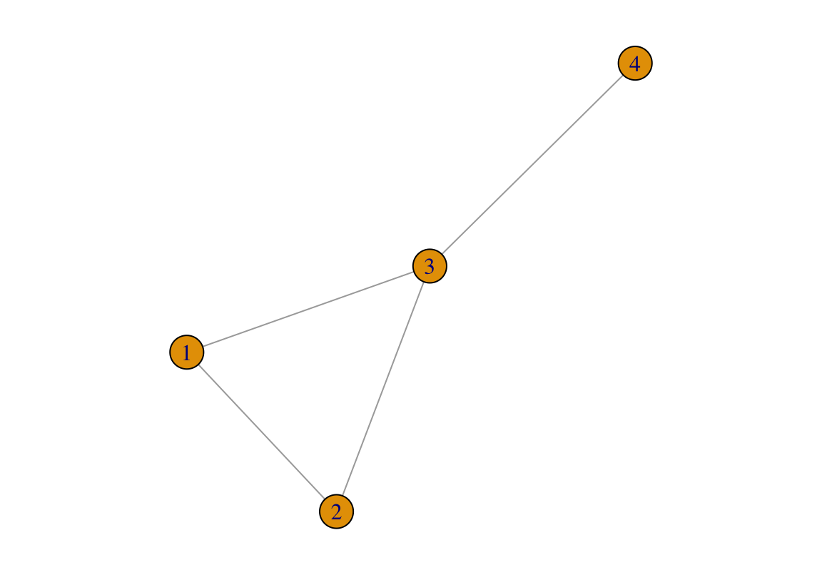
FIGURE 2.2: An undirected network for illustration.
For example, in the above network, nodes 1, 2, and 4 have a degree of two. Node 3 has a degree of three.
For the \(i^{th}\) node in a network, we’ll denote its degree as \(k_i\). Therefore, for the above network, \(k_1\)=\(k_2\)=\(k_4\)=2, \(k_3\)=3.
As mentioned above, the total number of links is denoted as L. In an undirected network, it is easy to understand that L should be half of the sum of all the node degrees. It should be halved because each link belongs to two nodes and therefore each is counted twice. We have:
\[\begin{equation} L = \frac{1}{2} \sum_{i=1}^N k_i \tag{2.1} \end{equation}\]
In the above network, \(L = 4\).
2.3.2 Average degree
Average degree, denoted as \(\langle k \rangle\) is simply the mean of all the node degrees in a network. For the network above (Figure 2.2), \(\langle k \rangle = \frac{1}{4} \cdot (k_1 + k_2 + k_3 + k_4) = \frac{1}{4} \cdot (2+2+3+2) = 2.25\). This means that on average, each node in the network has 2.25 links.
According to its definition, we know that \(\langle k \rangle\) = \(\frac{1}{N} \sum_{i=1}^N k_i\). Combined with Eq. (2.1), we have:
\[\begin{equation} \langle k \rangle = \frac{2L}{N} \tag{2.2} \end{equation}\]
How can we understand this equation?
I would understand it this way: we are calculating the average degree, so the denominator will be N, i.e., number of nodes, and the nominator will be the sum of all the nodes’ number of links, which should be \(2L\) because each link is shared by two nodes.
The above equation Eq. (2.2) is for undirected networks. What about directed networks? Should we calculate their average degree the same way?
g2 <- graph( edges=c(1,2, 1,3, 2,3, 3,4), n=4, directed=TRUE)
par(mar = c(1, 1, 1, 1))
plot(g2)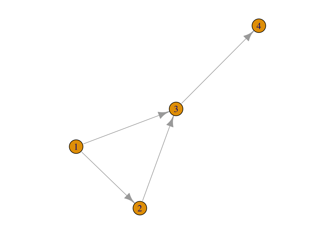
FIGURE 2.3: A directed network for illustration.
Each link in the above network (2.3) is directed. If we calculate the network’s average degree according to Eq. (2.2), we will be losing information.
Therefore, we will distinguish between incoming degree, denoted as \(k_i^{in}\) and outgoing degree, denoted as \(k_i^{out}\). \(k_i^{in}\) means the number of links from other nodes pointing to node \(i\), and \(k_i^{out}\) means the number of links starting from node \(i\) and pointing to other nodes.
For a given node \(i\) in a directed network, its degree is the sum of incoming degree and outgoing degree. Therefore,
\[\begin{equation} k_i = k_i^{in} + k_i^{out} \tag{2.3} \end{equation}\]
And L, the total number of links in a directed network, is:
\[\begin{equation} L = \sum_{i=1}^N k_i^{in} = \sum_{i=1}^N k_i^{out} \tag{2.4} \end{equation}\]
For a directed link between node i and node j, i.e., (i, j), it constitutes an incoming degree for one node, but an outgoing degree for the other. For example, in the network (2.3), (1,2) counts as an incoming degree for node 2, but an outgoing degree for node 1.
In fact, if we combine Eq. (2.3) with Eq. (2.4), we will know that Eq. (2.4) is equal to Eq. (2.1). Then why can’t we stick to Eq. (2.1) even for a directed network? This is because, I guess, we can have more information, i.e., incoming or outgoing degree, by using Eq. (2.4).
Last, what’s the average degree for a directed network?
We can definitely use Eq. (2.2), but, again, we will be missing valuable information. Therefore, we will distinguish between \(\langle k_{in} \rangle\) and \(\langle k_{out} \rangle\), the two of which, in fact, are equal:
\[\begin{equation} \begin{split} \langle k_{in} \rangle & = \frac{1}{N}\sum_{i=1}^N k_i^{in}\\ & = \langle k_{out} \rangle\\ & = \frac{1}{N}\sum_{i=1}^N k_i^{out}\\ & = \frac{L}{N} \end{split} \tag{2.5} \end{equation}\]
2.3.3 Degree distribution
In a large network, nodes’ degrees vary. For example, there might be 100 nodes with a degree of 10, 50 nodes with a degree of 9, 30 nodes with a degree of 7, etc.. Then what is the probability that a randomly picked node will have a degree of \(k\)?
Let’s denote this probability as \(p_k\), and call it as degree distribution, which, as is described above, is defined as “the probability that a randomly picked node in a network has a degree of \(k\).” According to this definition, we know that:
\[\begin{equation} p_k = \frac{N_k}{N} \tag{2.6} \end{equation}\]
where \(N_k\) represents the number nodes that have a degree of \(k\). From the equation above, we can infer that \(N_k = Np_k\)
We also know that since \(p_k\) is a probability, it should add up to 1:
\[\begin{equation} \sum_{i=1}^\infty p_k = 1 \tag{2.7} \end{equation}\]
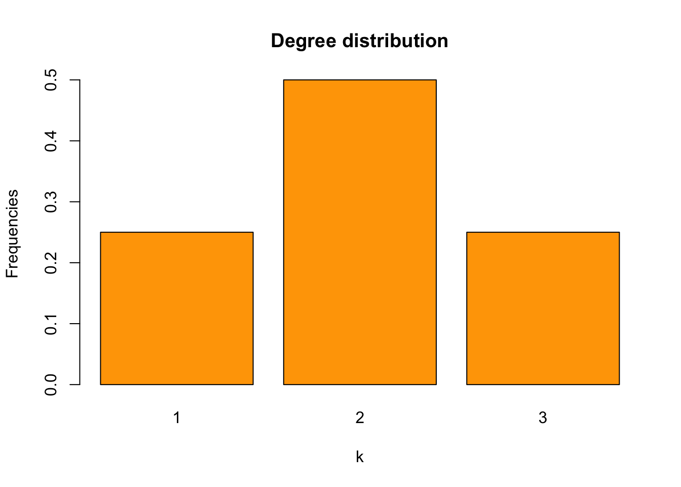
Take the network in Figure 2.2 as an example, its degree distribution is as follows: