5.3 The Barabási-Albert Model
The Barabási-Albert model, or BA model for short, addresses this question: how does a network’s degree distribution form a power law?
Two hidden assumptions of the random network model do not hold water in real networks:
The random network model assumes that the number of nodes is fixed. In real networks, however, this number continues to grow as new nodes join the network. That is to say, the size of a real network keeps growing.
The random network model assumes that a link is generated randomly. However, in real networks, new nodes prefer to link to high-degree nodes. This phenomenon is called preferential attachment.
The BA model recognized the coexistence of network growth and preferential attachment in real networks and proposed a method of generating networks with scale-free properties, i.e., hubs, and a degree distribution that follows a power law.
We begin with nodes. Each node’s degree is no less than 1. Links between these nodes are arbitrary.
At each timestep, a new node with a degree of () is added to the network.
The probability that node connects to an old node, denoted as node , is proportional to the old node’s degree (Menczer, Fortunato, and Davis 2020):
The denominator in Eq. (5.3) is the sum of all degrees in the old network, so the sum of all these probabilities is equal to one (Menczer, Fortunato, and Davis 2020).
The image 5.4 made me wonder whether my computation of 5.4 was wrong. I will check it later.
Update: Yeah, i was wrong. Originally, when calculatingdeg.dist_internet, I set cumulative to be FALSE. This is due to the fact that I did not quite understand power law distribution at that time. I need to set it to be TRUE.
5.3.1 Improving the BA model
Suppose you are an incoming node and are about to attach yourself to other nodes. According to Eq. (5.3), you first should calculate all the degree nodes in the existing network and then calculate the proportion of a specific node’s degree against the sum of all the degrees. This proportion will be the probability that you will connect to this node.
There is a problem in the first step. You need to know all the nodes before you can get the sum of all degrees. However, this is very difficult. For instance, when you enter a university, and are about to develop a friendship with other people, is it realistic for you to first know how many friends EVERY person at this university has? Probably not.
Is it possible for us to achieve preferential attachment without requiring knowledge about each and every node in the existing network?
Yes. Try this: The incoming node randomly chooses a link from the existing network, then connect to either end of this link. Hubs have more links connecting to it, so it is more likely for this incoming node to connect to a hub. If you have difficulty understanding why so, consider the extreme example of a star graph.
starG <- make_star(n = 12, mode = "undirected", center = 1 )
plot (starG)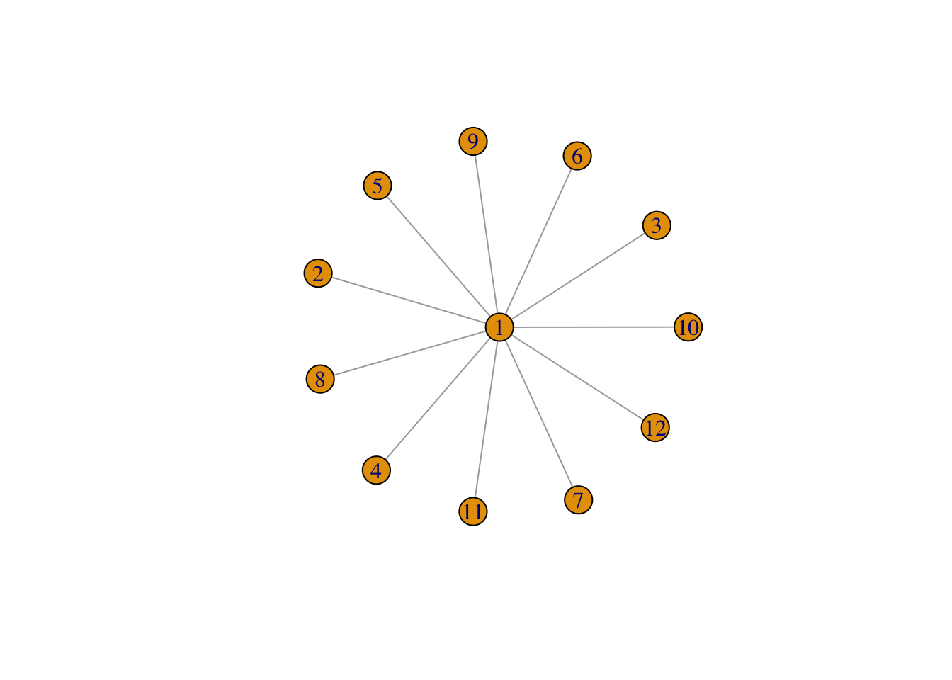
FIGURE 5.5: A star graph
In Fig. 5.5, no matter which link you pick, it is always connected to the hub.
If you have followed the understood the logic so far, you should be able to know that if (meaning node has twice as many links as node ), then the incoming node is twice as likely to connect to node . This means that the probability of connecting to node is linearly proportional to , which is how the BA model defines preferential attachment.