4.1 Random networks (Barabási Ch.3)
4.1.1 Generating a random network
Most of networks in real life look like randomly constructed. Then, how can we, as humans, produce random networks that we see in nature?
Simply by putting links randomly between nodes.
But how can we make sure that we are putting links randomly?
Think about it for a minute before reading on.
If you have studied statistics, you would know that randomness is all about probability. If we say that we are going to randomly pick a person from a group, then we’ll need to make sure that each person in the group has an equal chance to be picked. Otherwise, the choice is not random.
Now, let’s go back to our original problem: how can we randomly put links between nodes?
For example, we now have 100 isolated nodes, which are called singletons, as shown below. What to do next?
g4_1 <- graph( edges=NULL, n=100)
plot(g4_1)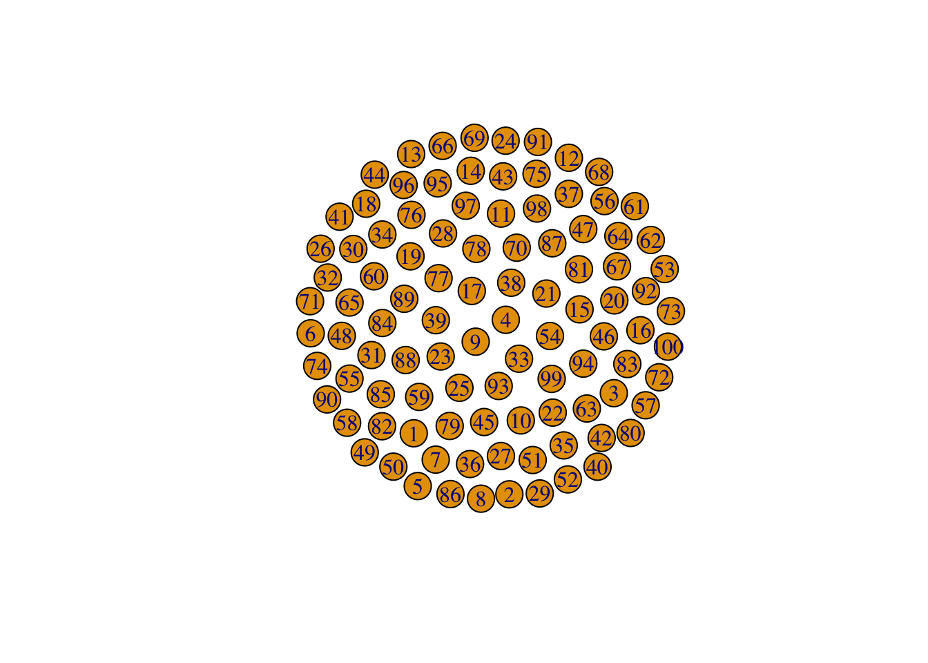
FIGURE 4.1: 100 isolated nodes
Frist, we’ll set up a value p (), called link probability. Then, we’ll pick a pair of nodes (STEP 1), for example, and , and generate a ramdom number for this pair (STEP 2). If , then we connect and . Otherwise, we keep them disconnected. We’ll repeat step 1 and step 2 for all node pairs, the total number of which should be . This way, we will make sure that the probability of each pair being connected is exactly . Why so?
plot(c(0, 1), c(0, 0.2),
     type= "n",
     xlab = "",
     ylab = "",
     yaxt="none")
# Solution: https://rstudio-pubs-static.s3.amazonaws.com/
# 297778_5fce298898d64c81a4127cf811a9d486.html
abline(v=0.1, col="red")
rect(0,0,0.1,0.2,col="lightgreen")
rect(0.1,0,1,0.2,col="red")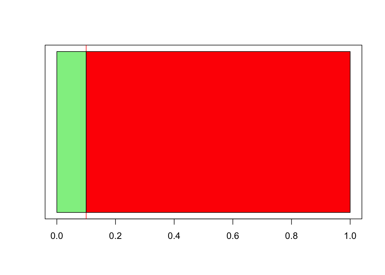
FIGURE 4.2: Illustrating why the probability of each pair being connected is equal to the link probability
The reason can be shown in Figure 4.2. If we set , then only of random numbers will fall in the range of (the area shown in light green), the remaining will fall in 1.
Okay, let’s set and see what will happen:
# Solution from: https://rpubs.com/lgadar/generate-graphs
set.seed(42)
erdosRenyi <- erdos.renyi.game(100, 0.1, type = "gnp")
plot(erdosRenyi)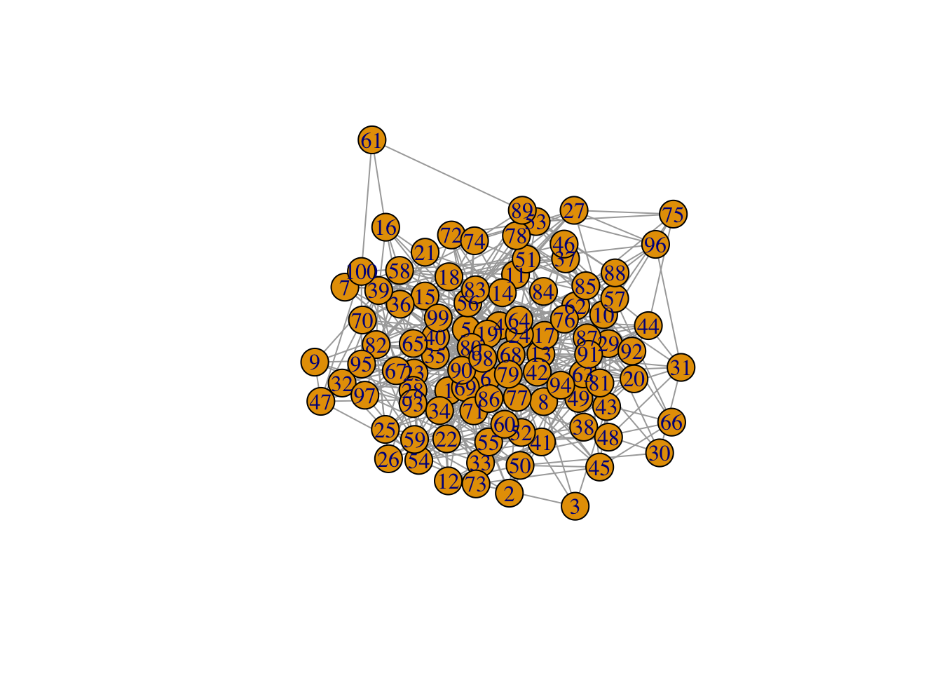
FIGURE 4.3: An Erdős-Rényi network
The method described above is used in a model called model, which was introduced independently by Edgar Nelson Gilbert. In this model, the number of nodes (), and link probability () are fixed.
There is a similar model called model where the number of nodes and the number of links are fixed. This model was introduced by Pál Erdős and Alfréd Rényi.
In practice, we use model more. But since Pál Erdős and Alfréd Rényi played such an important rold in advancing our understanding of random networks, we still name networks generated by the model as an Erdős-Rényi network.
4.1.2 Average degree, and the expected number of links in a random network
We can think of the process (of first generating a random number for a pair of nodes, then comparing it with , and finally deciding whether to link the pair or not) as tossing a coin (Menczer, Fortunato, and Davis 2020).
Imagine we have a biased coin which gives us heads with probability , which is equal to the link probability we talked about before. Take as an example. If we toss the coin for ten times, then we are expecting head, right? For the same token, when we have tosses, we will be expecting heads.
In the procudure of random network generation discussed above, we concluded that a pair of nodes being connected has a probability of , which is the same as the probability of us having a head when we toss a coin. Since we are expecting heads out of tosses, then how many connected pairs of nodes are expected, or, how many links are expected, if we examine pairs? , right?
How do we get this number? We simply multiply the total number of tosses in the case of flipping coins (or the total number of pairs of nodes we have in the case of random network generation) by . Now, in the model, we have nodes. It’s easy to understand that we will have pairs of nodes to examine. So, the number of links we are expecting in this random network is:
here stands for the expected value. A given random network generated by does not necessarily have exactly links. But as we generate more and more random networks using the model, the average number of links will be . That’s what we mean by expected value. You can look at Image 3.3 in Network Science for examples and illustrations.
Then, in this random network, what is the average degree?
Recall Eq. (2.2). Replacing with from Eq. (4.1), we have:
How to remember Eq. (4.2):
The average degree of a random network is the product of , the link probability, and , the maximum number of links (or neighbors) a node can have.You can read Ch. 3.3 of Network Science for more detailed mathematical reasoning.
4.1.3 Degree distribution
4.1.3.1 Binomial distribution
First of all, if you are not familiar with combinations and permutations, or that you have forgotten what you learnt in your high school, you are encouraged to go through this amazing tutorial on mathsisfun.com.
Then, carefully read throught this tutorial on binomial distribution.
If you are able to understand the tutorials above, then you should know that if we have a biased coin which produces heads with probability , the probability of having heads out of tosses is:
How to understand it?
We can look at it this way: tossing a coin times, we have different outcomes (i.e., combinations of heads and tails), and the number of outcomes (or combinations, if you want) that have heads is outcomes. However, we cannot simply use to calculate the probability of having heads. Why? Because this is a biased coin, so each outcome (or combination) has different probabilities.
What should we do then?
Now we know the number of outcomes that will produce heads out of tosses. It will be great if we know the probability of each of these outcomes and sum them up. Bingo!
When we think more deeply, we will know that each of these outcomes has exactly the same probability: . But why? Read this tutorial on binomial distribution again, especially the tree diagram. Also, you’ll find this tutorial on the probability of independent events helpful.
Now, let’s go back to random networks.
| random network generation | link probability | number of nodes | number of node pairs successfully connected |
| tossing coins | probability of having a head in one toss | number of tosses | number of heads |
For a given node , the maximum number of links it can have is . Let’s denote the probability of node having links as . Eq. (4.3), we know that:
In this binomial distribution, the mean is:
Its standard deviation is:
And its second moment is:
Sorry that I am currently not capable of proving Eq. (4.5) to Eq. (4.7). For now, just memorize them.
4.1.3.2 Poisson distribution
Most real networks are sparce, so its average degree is much smaller than the size of the network, . Considering this limit, we usually use Poisson distribution to describe a random network’s degree distribution because of simplicity:
Eq. (4.4) and Eq. (4.8) are collectively called degree dostribution of a random network.
Things to keep in mind:
Binomial form is the exact version; Poisson distribution is only an approximation;
We’d better use Binomial distribution to describe a small network, for example, , but use Poisson distribution for large networks, for example, or ;
In Poisson distribution, the standard deviation is ;
The Poisson distribution tells us that for two networks, as long as they have the same , their degree distribution is almost exactly the same despite different sizes, i.e., .
4.1.4 Poisson distribution does not capture reality
Poisson distribution undoutedly accurately describes the degree distribution of random networks, but we need to ask, do random netwoks reflect reality?
Reading Ch. 3.5, will let us know that if random networks can describe social networks in our daily lives, we would expect that:
Most people will have friends;
The highest number of friends a person can have is not that different than the smallest possible number.
However, we know that this is not the case in real life. Many people have over 5,000 contacts on Facebook and WeChat.
From the figure shown in Ch. 3.5, we will know that in real networks, both the number of high degree nodes, and the standard deviation of the distribution, are much larger than what is expected from random networks.
I am a little bit uncertain here because I don’t know where to put 0.1.↩︎