5.1 Power-Law Distributions
5.1.1 Differences between FB study and the Milgram study
The differences between the Facebook study and the Milgram study:
In FB study, researchers knew the whole graph. They would have this in mind when calculating the shortest paths. However, participants in the Milgram study did not know the whole graph;
There wasn’t any lost “packages” in FB study.
One thing we need to be cautious with the FB study is that there were quite a number of people having 500-5,000friends, as can be seen in the study PDF. But is it possible in real life? Dunbar’s number suggests that we as humans can maintain at most 150 friends. Therefore, the FB study might have overestimated the distance between people.
5.1.2 Power law
The above picture of the bird came from here.
Check out this video to understand Zipf’s law. Also, here is an amazing tutorial3 on the connection between Zipf’s law and power laws.
The most frequently used word in English is the. Let’s denote its frequency as . Then the frequency of the second most frequently used word is . The number is for the third most frequently used word, and will be for the fourth most frequently used word. That’s a power law distribution.
5.1.3 Logarithmic scale
To really understand scale free networks and power law distribution, we need to get an idea of logarithmic scale first. Professor YY provided several very helpful Youtube videos that illustrate log scale.
Inspired by the conversation between Vi and Sal, I am asking you this question. In the following number line, from to 1 million, where is ?

Okay, let’s label both and in the above number line:
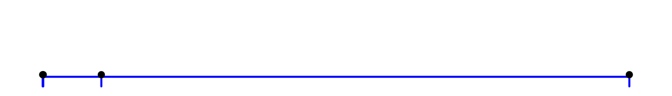
I plotted four points: 0, 1000, 100000, and 1000000, but can only see three. Why? It’s because 0 and 1000 are almost at the same place. But I guess you’ve probably thought was in the place of , right?
You can learn some basics of log scale by watching this video by Khan Academy.
One of the reasons why people need log scale is that it allows us to include a much wider range of numbers in limited space. For example, it is useful when we measure earthquakes.
5.1.4 Properties of power-law distributions
5.1.4.1 Porperty 1: A fat tail allowing for many outliers
A power-law distribution can be expressed as
where > 1.4
If we take a logarithm of Eq. (5.1), we’ll have
If you are not familiar with or how the above calculations are done, do read this tutorial on logarithm.
If , then, , where , , and . In this example, is called base of the logarithm.
- If the base is : will be denoted as
- If the base is : will be denoted as
Some logarithmic identities:
- ;
- ;
- ;
Since is a constant, what we get is basically a linear function. To better understand it, let’s plot it.
Before we take the log:
x <- 1:100
y <- 5*x^(-2)
plot (x, y, pch=19, cex=0.5, col="orange",
      xlab="X", ylab="5*x^(-2)",
      main="Before taking a log")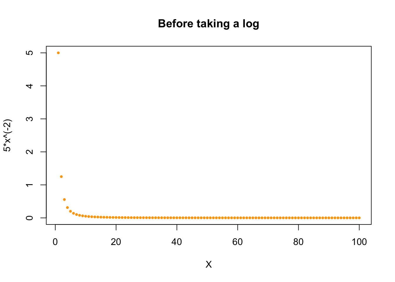
I learned a lot about how to style the points from reading Dr.Katya Ognyanova’s blog post.
If we take a log:
x <- 1:100
y <- 5*x^(-2)
plot (x, y, pch=19, cex=0.5, col="orange",
      xlab="log(X)", ylab="log(Y)",
      main="After taking a log",
      log="xy"
      )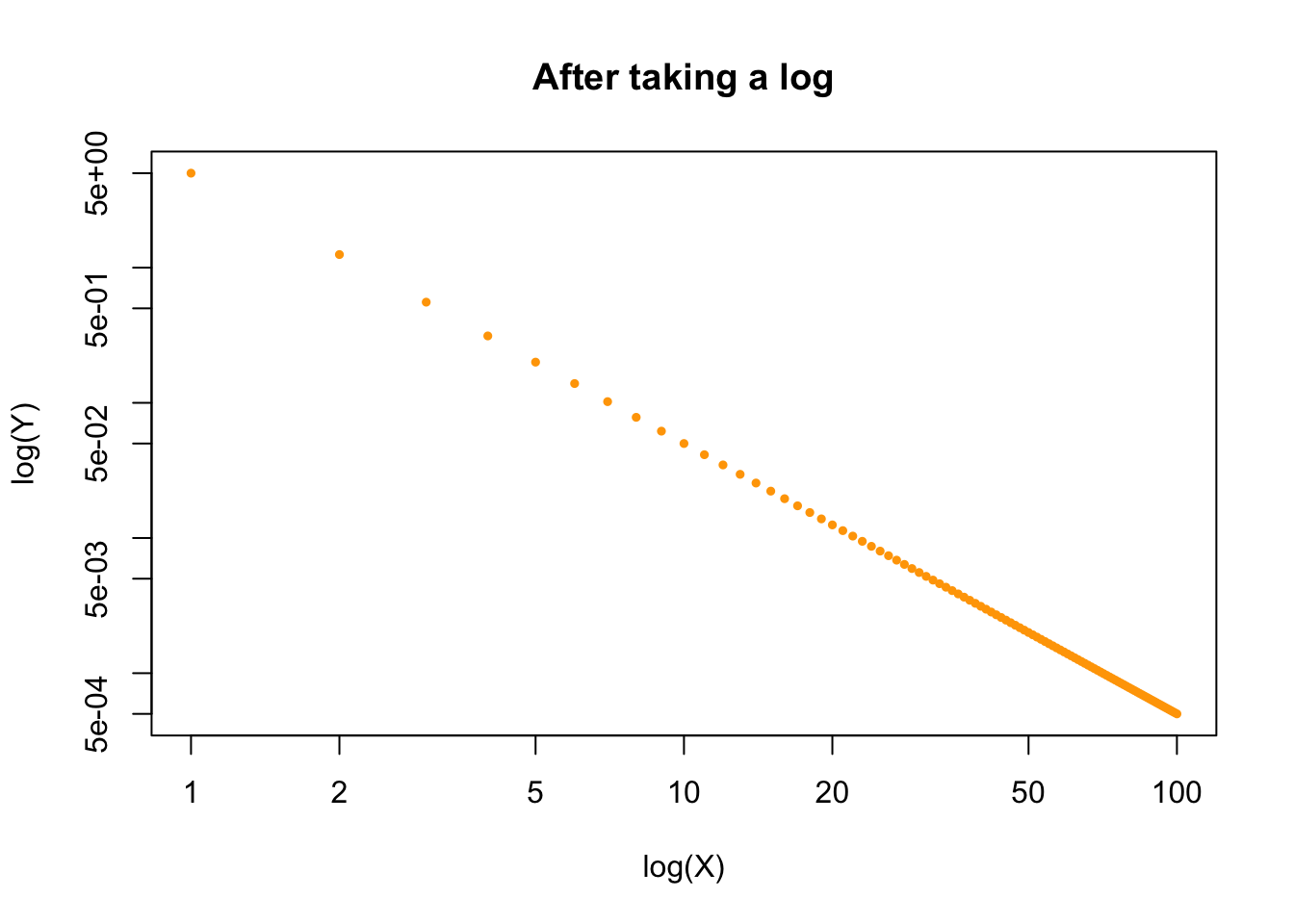
A very important property of power-law distribution on a log-log scale is it has a heavy tail or a so-called fat tail. Lots of other distributions, like binomial, Poisson, or normal distributions, simply do not have this fat tail, which is super useful when we have lots of outliers in the tail of the distribution.
As we can clearly see below, except for the power-law distribution on a log-log scale, in all the three other distributions, quickly reaches zero:
par(mfrow=c(2,2))
# The idea of the following codes comes from
# https://www.statology.org/plot-normal-distribution-r/
x_dnorm <- seq(-6, 6, length=100)
y_dnorm <- dnorm(x_dnorm)
plot(x_dnorm, y_dnorm, pch=19, cex=0.5, col="skyblue",
     main="Normal Distribution")
# The following codes are from
# https://www.tutorialspoint.com/r/r_binomial_distribution.htm
x_dbinom <- seq(0,50,by = 1)
y_dbinom <- dbinom(x_dbinom,50,0.5)
plot(x_dbinom, y_dbinom, pch=19, cex=0.5, col="red",
     main = "Binomail Distribution")
# The following codes are from https://statisticsglobe.com/poisson-
# distribution-in-r-dpois-ppois-qpois-rpois
x_dpois <- seq(-5, 50, by = 1)
y_dpois <- dpois(x_dpois, lambda = 10)
plot(x_dpois, y_dpois, pch=19, cex=0.5, col="purple",
     main = "Poisson Distribution")
x <- 1:100
y <- 5*x^(-2)
plot (x, y, pch=19, cex=0.5, col="orange",
      xlab="log(X)", ylab="log(Y)",
      main="Power-law Distribution (Log-Log Scale)",
      log="xy")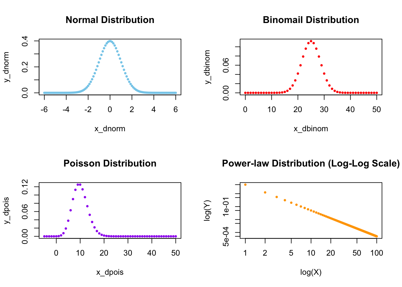
FIGURE 5.1: Comparing Four Different Distributions
If we have many outliers in the tail, for example, in the household income distribution shown below by Donovan, Labonte, and Dalaker (2016), which of the four distributions shown above will you choose to fit the income distribution? Definitely we’ll use the power-law distribution which has a fat tail.
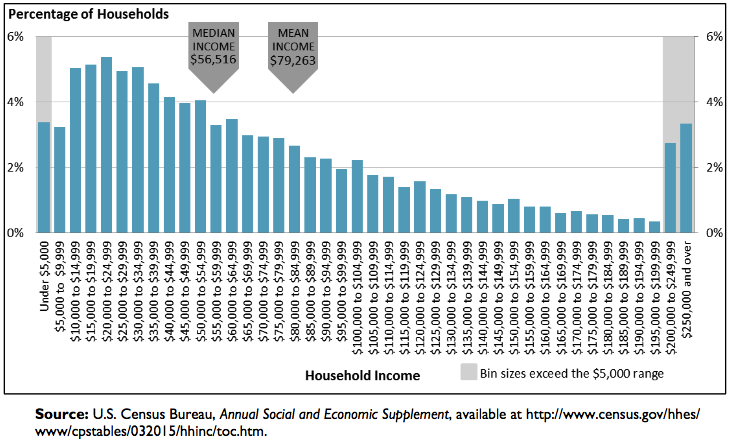
FIGURE 5.2: US Household Income Distribution in 2015, Visualization by Donovan, Labonte, and Dalaker (2016)
We can also compare a normal distribution and a power-law distribution side by side:
par(mfrow=c(2,1))
x_dnorm_2 <- seq (0, 10000, by = 1)
y_dnorm_2 <-dnorm(x_dnorm_2)
plot (x_dnorm_2, y_dnorm_2, pch=19, cex=0.1, col="blue",
      xlab="x_dnorm", ylab="y_dnorm",
      main="Normal Distribution")
x <- 0:10000
y <- 5*x^(-2)
plot (x, y, pch=19, cex=0.1, col="orange",
      xlab="log(X)", ylab="log(Y)",
      main="Power-law Distribution (Log-Log Scale)",
      log="xy")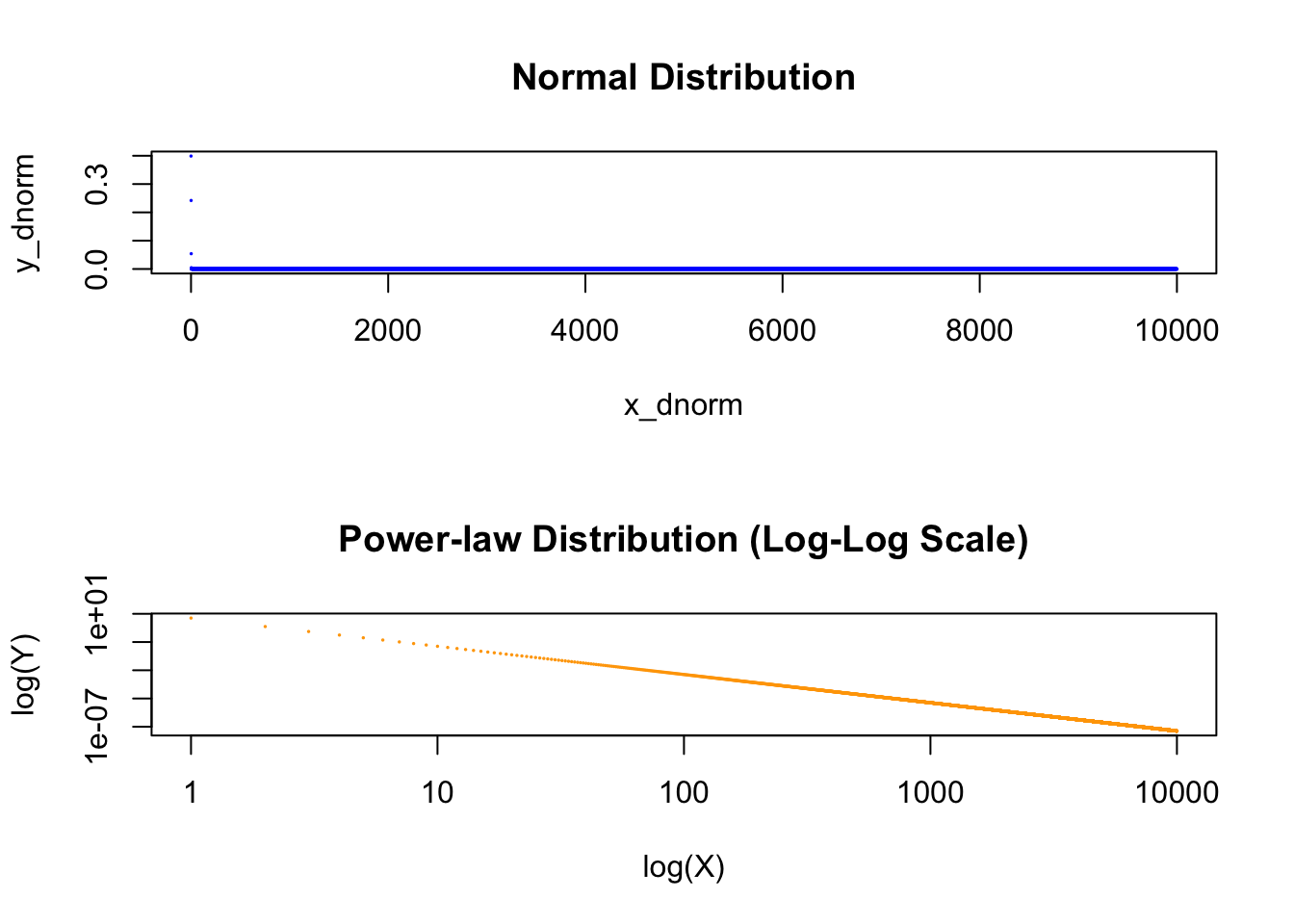
FIGURE 5.3: Comparing Normal Distribution and Power-law Distribution Side by Side
In power-law distribution plotted on a log-log scale, we do expect a lot of outliers.
5.1.4.1.1 Property 2: scale-freeness
To deeply understand what the term “scale-free” means, you can read Chapter 4.4 in Network Science.
I’ll explain in my own words here. To understand “scale-free,” we must first understand “scale.” Mark Newman (2005) defines it this way: A scale is "a typical value around which individual elements are centered (p.1). Therefore, scale-free means that we don’t know around which value individual elements in the distribution are centered. A normal distribution is not scale-free because we expect that more than 99% of the data falls within three standard deviations from the mean.
You can read Power laws, Pareto distributions and Zipf’s law by Mark Newman (2005) for details. This paper is also a must read if you want to gain a deeper understanding about power law.)
In a power-law distribution, it’s totally different. For example, if we have . Let’s imagine that human height follows this distribution. Suppose your height is , and people have the same height as you. Then you’ll see people twice as tall as you5, and people half of your size. The thing is, you don’t know where you are located in the distribution! You can be as tiny as inches or as tall as feet. Wherever you stand, you will always find people twice as tall as you, and people half of your size. Think about it! What a crazy world! That’s why we call it scale-free: no inherent scale in the distribution.
I haven’t throughly read and understood it yet…↩︎
Read here for why: http://tuvalu.santafe.edu/~aaronc/courses/7000/csci7000-001_2011_L2.pdf.↩︎
Just input in the above formula.↩︎