5.2 Scale-free property
In real networks, there are hubs that are forbidden in random networks.
No matter what properties of a network we are studying, we need to base our understanding on the network’s degree distribution.
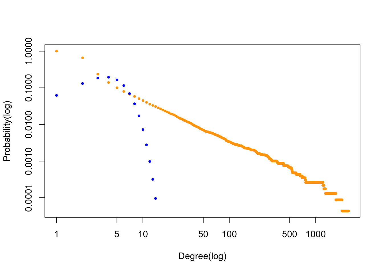
The book compares the Poisson distribution and power-law distribution by drawing the degree distribution of the WWW. I wanted to understand these two distributions better so I decided to try drawing them by myself.
The data I used is called “Internet” from http://www-personal.umich.edu/~mejn/netdata/. I’ll use R to plot it. See the result in Figure 5.4
library(here)
internet <- read_graph(here("data","as-22july06.gml"),
                       format = "gml")
# vcount(internet) # Getting an idea of its size // 22963
deg_internet <- degree(internet)
# mean(deg_internet) # Calculating average degree // 4.218613
x <- 0:max(deg_internet) # Setting X-axis
deg.dist_internet <- degree_distribution(internet,
                                         cumulative = TRUE,
                                         mode = "all")
# This will be the degree distribution of our dataset:
y1 <- deg.dist_internet
y2 <- dpois(x, lambda = mean(deg_internet))
# This is to prevent scientific notation on the axes:
options(scipen = 5)
plot( x, y1, pch=19, cex=0.5,
      col="orange",
      xlab="Degree(log)",
      ylab="Probability(log)",
      log = "xy"
      )
# par(new=TRUE)
points(x, y2, pch=19,
     cex=0.5,
     # log = "xy", # We can, in fact, do without this line
     # because the above plot is already on a log-log scale.
     col="blue",
     xlab = "",
     ylab = ""
     )
FIGURE 5.4: Poisson distribution does not explain degree distribution in real networks
The above code is based on this post.
We can see that the degree distribution of the real network is different from Poisson distribution but rather roughly follows a power law. We call networks like this as scale-free networks.
A quick note: in the above codes, y2 <- dpois(x, lambda = mean(deg_internet)) ensures that both networks share the same . Therefore, the result in the figure tells us that the degree distribution of this real network cannot be approximated by Poisson distribution.
5.2.1 Hubs
Hubs are nodes with high degrees. To understand that there are more hubs in scale-free networks than in random networks, we can refer to Figure 5.4. The two distributions have exactly the same average degree, .
We will find that compared to random networks, scale-free networks have more low-degree nodes and high-degree nodes, but fewer nodes with degrees near the average degree. This tells us that in random networks, most nodes have comparable degrees (around the average degree of the network) whereas in scale-free networks, there are so many nodes with extremely low and extremely high degrees.
Another difference lies in how the maximum degree (denoted as ) changes as the size of networks increases. For both types of networks, grows as becomes larger. The difference is that grows faster (polynomially) with in scale-free networks but it grows slower (logarithmatically) in random networks. Also, if a random network and a scale-free network has the same average degree , the in the scale-free network is almost always larger than that in the random network.
Read the section of The Largest Hub in Chapter 4.3 for formula derivation. I am currently not capable of doing it.
5.2.2 Universality
Both World Wide Web (WWW) and the Internet are networks. WWW is a network of information. Its nodes are documents and its links are URLs. In contrast, the Internet is a network of infrastructure. Its nodes are computers and its links are cables and wireless connections. Although they are different, their degree distribution can be both approximated with a power law, meaning that there are a large amount of high degree nodes (“hubs”) and low degree nodes. In other words, both reveal scale-free properties.
Since scale-free properties are so prevalent, we call scale-free property a universal characteristic for networks.
As ubiquitous as it is, the scale-free property isn’t for every networks. Many networks do not share this property, for example, power grid and material networks. Scale-freeness requires that the number of links a node can have is arbitrary, and not systematically constrained. If this requirement is not fulfilled, then hubs are restricted and the network won’t show a scale-free property.
5.2.3 Ultra-small property, and the role of degree exponent
Small-world property is the only characteristic in real networks that is well explained by random network models, more specifically, by the Watts-Strogatz model.